The upper limit of a network’s capacity is its liquid throughput. The liquid throughput corresponds to the flow of a liquid in an equivalent network of pipes. In coarse-grained networks, the aggregate throughput of an arbitrarily scheduled collective communication may be several times lower than the maximal potential throughput of the network. In wormhole and wavelength division optical networks, there is a significant loss of performance due to congestions between simultaneous transfers sharing a common communication resource. We propose to schedule the transfers of a traffic according to a schedule yielding the liquid throughput. Such a schedule, called liquid schedule, relies on the knowledge of the underlying network topology and ensures an optimal utilization of all bottleneck links. To build a liquid schedule, we partition the traffic into time frames comprising mutually non-congesting transfers keeping all bottleneck links busy during all time frames. The search for mutually non-congesting transfers utilizing all bottleneck links is of exponential complexity. We present an efficient algorithm which non-redundantly traverses the search space. We efficiently reduce the search space without affecting the solution space. The liquid schedules for small problems (up to hundred nodes) can be found in a fraction of seconds.

1. Introduction

1.1.Parallel transmissions in circuit-switched networks

It’s been more than three decades that circuit-switched networks are being successfully replaced by their packet-switched counterparts. In early 1970’s this trend started by replacing data modems with connections to the X.25 network. Today, the entire telephony is being packetized. It is commonly admitted that with fine-grained packet-switching technology, network resources are utilized more efficiently, flows are more fluid and resilient to congestions, network management is easier and the networks can flexibly scale to large sizes.

Nevertheless, several other networking approaches still based on coarse-grained circuit-switching have been emerging. These approaches offer low latencies, which is not attainable with packet switching technology, but they are also arising due to technological limitations (in optical domain).

Examples of such networks are wormhole and cut-through switching (e.g. MYRINET, InfiniBand) and optical Wavelength Division Multiplexing (WDM). Both, in wormhole and optical switching, the number of network hops separating the end nodes has nearly no impact on the communication latency (in contrast to packet switching). As for optical networks, due to the lack of optical memory, packet switching in optical networks does today not exist at all (at least commercially).

All coarse-grained circuit-switching networks suffer from a common problem: inter-blocking of transfers and jamming of large indivisible messages occupying intersecting fractions of network resources. Several parallel multi-hop transmissions cannot share the same link resource simultaneously. In contrast to the fluidity and resiliency of packet-switching, in coarse-grained circuit-switching networks hard and complex interlocking contentions arise when the network topology grows and the load increases.

In WDM optical networks, a single fiber can carry several wavelengths (about 80 in WDM, 160 in DWDM and about 1000 in research [Kartalopoulos00]). However the contentions are still present, because the wavelengths are typically conserved along the whole communication path between the end nodes (no switching from one wavelength to another occurs in the middle of the network). The new wavelengths are simply increasing the network capacity. In subsection 2.2 we give a brief introduction to the WDM wavelength routing technology. In wormhole switching, when the head of the message is blocked at an intermediate switch (due to contention), the transmission stays strung over the network, potentially blocking other messages. The wormhole routing technology is briefly described in subsection 2.1.

1.2.Hardware solutions

In optical and wormhole switching the problem of contentions can be solved partially or fully at the hardware level.

For example the optical switches of the network may be equipped with the capability to change the incoming wavelengths (not only to switch across the ports, i.e. to control the direction of the light, but also to change the wavelength). Wavelength interchange (changing of colors) requires expensive optical-electric (O/E) and electro-optical (E/O) conversions. Without O/E/O conversions, when the signal is constantly maintained in the optical domain, cost-effective optical networks can be built by relying only on switching by microscopic mirrors, using inexpensive Micro Electro-Mechanical Systems (MEMS). In addition, O/E/O conversions necessarily induce additional delays.

Regarding wormhole routing, the switches typically need only to buffer the tiny piece of the message (flit) that is sent between the switches. However, the switches can be equipped with memories large enough to store the entire message (whichever is the estimation of the message size in the network). Thus, when the head of the message is blocked, the switch lets the tail continue, accumulating the whole message into a single switch. This hardware extension changes the name of the wormhole routing into cut-through switching. Storing of the messages solves the contention problem only partially but requires a substantial increase of the switch’s memory, up to multiples of the largest message size (depending on the number of ports). Virtual cut-through switching is yet another hardware extension, where the link is divided (similarly to WDM) into a certain number of virtual links sharing the capacity of the physical link.

The hardware solutions of contention-avoidance in coarse-grained switching require costly modifications of hardware (e.g. O/E/O conversion in optical switching or substantial memory in wormhole switches) and often only provide partial solutions. The hardware solutions not only induce additional cost, but reduce the benefits of important properties of the coarse-grained networks, such as the low latency (e.g. by storing entire messages in cut-through switches).

1.3.Liquid scheduling - an application level solution

In wormhole routing, for example, by keeping the architecture simple, switches with a large number of physical ports can be implemented in single chips at very low cost. Liquid scheduling is an application level method for achieving the network’s best overall throughput. The scheduling is performed at the edge nodes and requires no specific hardware solutions. Synchronization and coordination of edge nodes is required.

Numerous applications rely on coarse-grained circuit-switched networks and require an efficient use of network resources for collective communications. Such applications comprise parallel acquisition and distribution of multiple video streams [Chan01], [Sitaram00], switching of simultaneous voice communication sessions [H323], [EWSD04], [SIP], and high energy physics, where particle collision events need to be transmitted from a large number of detectors and filters to clusters of processing nodes [CERN04].

Liquid scheduling can be used in Optical Burst Switching (OBS) by the edge IP routers for efficient utilization of the capacities of an interconnecting optical cloud (all-optical network providing interconnection for the edge routers).

1.4.Overview of liquid scheduling

The aggregate throughput of a collective communication pattern (traffic of transmissions between pairs of end nodes) depends on the underlying network topology and the routing. The amount of data that has to pass across the most loaded links of the network, called bottleneck links, gives their utilization time. The total size of a traffic divided by the utilization time of one bottleneck link gives an estimation of the liquid throughput, which corresponds to the flow capacity of a non-compressible fluid in a network of pipes [Melamed00]. Both in wormhole switching networks and WDM optical networks, due to possible link or wavelength allocation conflicts, not any combination of transfer requests may be carried out simultaneously. The objective is to minimize the number of timeslots and/or wavelengths required to carry out a given set of transfer requests. Each transfer shall be allocated to one (and only one) time frame, such that no pair of transfers allocated to the same time frame uses a common resource (link, wavelength). The liquid scheduling problem is introduced and mathematically defined in sections 3 and 4.

The liquid scheduling problem cannot be solved in polynomial time. Solving the problem by Mixed Integer Linear Programming (MILP) [CPLEX02], [Fourer03] requires very long computation time (see Appendix B). Solving the problem by applying a heuristic graph coloring algorithm provides in short time suboptimal solutions. The throughputs corresponding to the heuristic solutions of the graph coloring problem are often 10% to 20% lower than the liquid throughput [Gabrielyan03] (see Appendix A). In the present contribution we propose an exact method for computing liquid schedules, which is fast enough for real time scheduling of traffics on small size networks comprising up to hundred nodes.

Section 2 is a brief overview of the architectures of the optical and wormhole switching networks. Sections 3 and 4 contain definitions. Sections 5, 6 and 7 introduce the liquid schedule construction algorithm. In section 8 we introduce several hundreds of traffic patterns across a real network and we present their overall communication throughputs when carried out according both, liquid schedules and topology-unaware schedules. This chapter is concluded by section 9.

2. Applicable networks

This section briefly introduces the basic architectures of two coarse-grained switching concepts: wormhole switching (subsection 2.1) and lightpath routing (subsection 2.2). The advantages of applying liquid scheduling are discussed for both types of networks.

2.1.Wormhole routing

Wormhole routing is used in many High Performance Computing (HPC) networks. In wormhole routing, the links lying on the path of a message are kept occupied during the transmission of that message. Unlike packet switching (or store-and-forward switching) where each network packet is present at an intermediate router [Ayad97], wormhole switching [Liu01], [Dvorak05] transmits a message as a “worm” propagating itself across intermediate switches. The message “worm” is a continuous stream of bits which are making their way through successive switches. In a wormhole switching network [Duato99], [Shin96], [Rexford96], [Colajanni99], [Dvorak05] a message entering into the network is being broken up into small parts of equal size called flits (standing from flow-control digits). These flits are streamed across the network. All the flits of a packet follow the same path. The head flit contains the routing header for the entire message. As soon as a switch on the path of a message receives the head flit, it can trigger the incoming flow to the corresponding outgoing link. If the message encounters a busy outgoing link, the wormhole switch stalls the message in the network along the already established path until the link becomes available. Occupied channels are not released. A channel is released only when the last tail flit of the message has been transmitted. Thus each link laying on the path of the message is kept occupied during the whole transmission time of a message. In virtual cut-through (VCT) networks, if the message encounters a busy outgoing link, the entire message is buffered in the router and already allocated portions of the message path are released. In VCT switches have enough memory to store as many messages of the maximal size as number of ports. Simple wormhole switch architecture which is only pipelining the messages and requires not more than a very small buffer, enables a cost effective implementation of large scale wormhole switches on a single chip [Yocum97]. The ability of VCT switches to buffer large messages increases their cost substantially.

Compared with store and forward switches, wormhole switching considerably decreases the latency of message transmission across multiple routers. Wormhole switching makes the latency insensitive to the distance between the end nodes. Most contemporary research and high-performance commercial multi-computers use some form of wormhole or cut-through networks, e.g. Myrinet [Boden95], fat tree interconnections for clusters [Petrini01], [Petrini03], [Quadrics], InfiniBand [InfiniBand], [Steen05], and Tnet [Horst95], [Brauss99B].

Due to blocked message paths, wormhole switching quickly saturates as load increases. Aggregate throughput can be considerably lower than the liquid throughput offered by the network. The rate of network congestions significantly varies depending in which order the same set of message transfers is carried out. Liquid scheduling enables partitioning of the transfers so as to avoid transmission of congesting messages at the same time.

2.2.Optical networks

In optical networks, data is transferred by lightpaths. Lightpaths are end to end optical connections from a source node to a destination node. In Wavelength Division Multiplexing (WDM) optical networks, a lightpath is typically established over a single wavelength (color) along the whole path. Different lightpaths in a WDM wavelength-routing network can use the same wavelength as long as they do not share any common link. Figure 1 shows an example of an optical wavelength-routing network. Switches of the optical network are called Optical Cross Connects (OXC). An OXC switches wavelengths from one port to another, usually without changing the color [Ramaswami97], [Stern99]. The Optical Line Terminal (OLT) multiplexes multiple wavelengths into a single fiber and de-multiplexes a set of wavelengths from a single fiber into separate fibers. Often the OLT units are integrated with OXC.

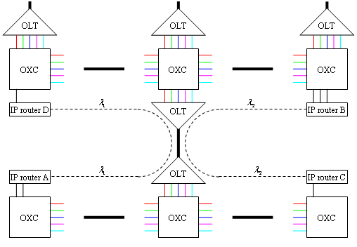
Figure 1. Wavelength routing in optical layer

End nodes (or edge nodes) of an optical network (also called optical cloud) are IP routers, SONET terminals or ATM switches. They are plugged to OXC switches (as shown in Figure 1). In a simple design the end node can be also inserted into a fiber (statically) via an Optical Add/Drop Multiplexer (OADM). The purpose of the optical cloud is to provide lightpaths between the terminal edge nodes, for example between IP routers (as shown in Figure 1). The lightpaths between the end nodes can be established either permanently, or provided dynamically on demand.

Relatively inexpensive OXC switches can be implemented by an array of microscopic mirrors, build with Micro Electro-Mechanical Systems (MEMS). These switches only re-direct the incoming wavelengths to appropriate outgoing ports, without converting the color. They are called Wavelength-Selective Cross-Connect (WSXC). Changing of the wavelength is possible through Optical/Electro/Optical (O/E/O) conversions. Optical switches providing wavelength conversion features are called Wavelength-Interchanging Cross-Connects (WIXC). WIXC switches do both space switching and wavelength conversion.

When using WIXC switches, the lightpaths may be converted from one wavelength to another along their route. However from the optical network design point of view, it is essential to keep transmissions in the optical domain as long as possible, i.e. to be able to provide the required services using only inexpensive WSXC switches.

Wavelength continuity (the fact that the basic optical transmission channel remains on a fixed wavelength from end to end) is the main constraint affecting the scalability of networks built with WSCX switches only.

For example assuming only WSXC switches in Figure 1, two connections from IP router A to B and from C to D must either be established on two different wavelengths and , or must be scheduled in different timeslots.

Given that any lightpath must be assigned the same wavelength on all the links it traverses and that two lightpaths traversing a common link must be assigned different wavelengths, the wavelength assignment problem requires minimizing of the number of wavelengths needed for establishment of the required end to end connections. In this domain, the wavelength assignment problem is commonly solved by solving the corresponding congestion graph coloring problem [Bermond96], [Caragiannis02]. The vertices of the graph represent the lightpaths and two vertices are connected if the corresponding lightpaths are sharing a common link. The graph coloring problem requires coloring of all vertices using a minimal number of colors such that two connected vertices always have different colors. Graph coloring is an NP-complete problem. Its solutions are generally based on heuristic methods.

Liquid scheduling is an efficient method for assigning transmissions a minimal number of lightpaths or timeframes. If a liquid schedule exists, the solution of the liquid scheduling algorithm corresponds to the optimal solution of the graph coloring algorithm. Our algorithm does not associate the set of transfers with a graph. It does not only consider the congestion between pairs of transfers (congestion graph) but also considers the set of links occupied by each transfer. This permits to build liquid schedules relatively fast for networks comprising up to hundred nodes. The corresponding congestion graphs comprise thousands of vertices. The heuristic graph coloring algorithms often propose solutions requiring more timeframes than the number of timeframes allocated by our liquid scheduling algorithm. The comparison of the liquid scheduling algorithm with a heuristic graph coloring method is given in Appendix A.

Application of liquid schedules in the optical domain assumes a collaboration of the edge nodes and therefore an appropriate signaling layer. Optical Burst Switching (OBS) is an example where the collaboration of the edge nodes is assumed and the application of a liquid schedules may significantly improve the overall throughput of the optical cloud [Qiao99], [Turner99], [Turner02]. In a scenario for a continuous incoming IP traffic, the continuously filled buffers of the edge nodes are repeatedly emptied by applying liquid scheduling. For the buffered data, the liquid schedule finds the minimal number of partitions comprising non-congesting lightpaths. The same wavelength is allocated to all transfers of a partition. The number of wavelengths available in the network may not suffice for all partitions found by the liquid schedule. In such a case, when all transfers cannot be carried out within a single round (timeslot), new rounds (with a new set of wavelengths) are allocated until all transfers are carried out. Irrespectively of the number of wavelengths available in the network, liquid scheduling minimizes the total number of required rounds.

Local strategies for avoiding congestions rely on an admission control mechanism [Jagannathan02], [Mandjes02] or on feed-back and flow control based mechanisms regulating the sending nodes’ data rate [Maach04], [Chiu89], [Loh96]. These mechanisms permit to avoid congestions by rejecting the extra traffic. Local decisions based strategies are utilizing only a fraction of the network’s overall capacities. The global liquid scheduling strategy ensures that the network’s potential capacities are used efficiently.

3. The liquid scheduling problem

In our model, we neglect network latencies, we consider a constant message (or packet) size, an identical link throughput for all links and assume a static routing scheme.

Consider a simple network example consisting of ten end nodes , , two wormhole cut-through switches , and twelve unidirectional links , , , all having identical throughputs (see Figure 2). Assume that the nodes are only transmitting and the nodes are only receiving. The routing is straight-forward, e.g. a message from to traverse links , and , a message from to uses only links and , etc.

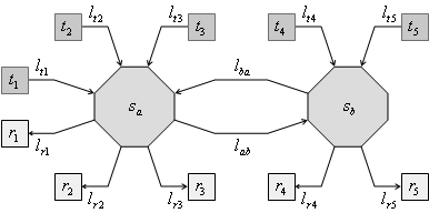
Figure 2. A simple network sample

For demonstration purposes we represent the transfers of the network of Figure 2, symbolically via small pictograms highlighting the links used by the transfer. For example the transfer from to is symbolically represented as , the transfer from to as . We may also represent a set of two or more simultaneous transfers by a pictogram highlighting all occupied links. For example a simultaneous transmission of the two previous transfers (from to and from to ) is represented as .

We are assuming that all messages have identical sizes [Naghshineh93]. Let each sending node have messages to be transmitted to each receiving node. There are therefore 25 transfers to carry out. These corresponding pictograms for these 25 transfers are shown in

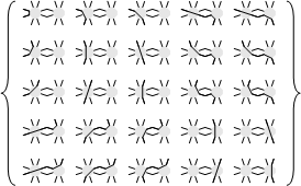
Figure 3. The pictograms representing the 25 transfers from all sending nodes to all receiving nodes of the network of Figure 2

Accordingly, each of the ten links , must carry 5 transfers, but the two links , must each carry 6 transfers. Therefore, for the 25 transfers to carry out, the links , are the network bottlenecks and have the longest active time. If the duration of the whole communication is as long as the active time of the bottleneck links, we say that the collective communication reaches its liquid throughput. In that case the bottleneck links are obviously kept busy all the time along the duration of the communication traffic. Assume in this example a single link throughput of 1Gbps. The liquid throughput offered by the network is .

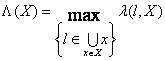
The liquid throughput of a traffic X is the ratio multiplied by the single link throughput (identical for all links), where is the total number of transfers and is the number of transfers carried out by one bottleneck link (the messages have identical sizes).

Now let us see if the order in which the transfers are carried out in this network has an impact on the overall communication throughput. A straight forward schedule allowing to carry out these 25 transfers is the round-robin schedule. At first, each transmitting node sends the message to the receiving node staying in front of it, then to the receiving node staying at the next position, etc. Such a round robin schedule consists of 5 phases.

The transfers of the first , second and the fifth phases of the round-robin schedule may be carried out simultaneously, but the third phase , , , , and the forth phase , , , , contain congesting transfers. For example, the two transfers of the third phase: and , cannot be carried out at the same time since they are trying to simultaneously use link (see Figure 2). Similarly, two other transfers of the third phase , are also in congestion, since they are simultaneously competing for the same link . The forth phase of the round-robin schedule has two pairs of congesting transfers as well. Each of these phases cannot be carried out in less than two time frames and therefore the whole schedule lasts 7 time frames and not 5 (the number of phases in the round-robin schedule). Five timeframes could have been sufficient if there were additional capacities (links) between the switches and . The throughput of the collective communication carried out according to the round-robin schedule is messages per time frame, or , which is below the liquid throughput of 4.17Gbps.

The 25 transfers can be scheduled within a fewer number of timeframes. The following schedule , , , , , carries out the 25 transmissions in 6 timeframes. Each timeframe consists of 3 to 5 non-congesting transfers. The whole schedule is yielding the liquid throughput of 4.17Gbps.

In the following sections we present algorithms permitting the construction of liquid schedules for arbitrary traffic patterns on arbitrary network topologies.

4. Definitions

The method we propose allows us to efficiently build liquid schedules for non-trivial network topologies. Thanks to liquid schedules we may considerably increase the collective data exchange throughputs, compared with traditional topology unaware schedules such as round-robin or random schedules.

The present section introduces the definitions that will be further used for describing the liquid schedule construction method.

A single “point-to-point” transfer is represented by the set of communication links forming the network path between one transmitting and one receiving node according to the given routing. Note that we will be limiting ourselves to data exchanges consisting of identical message sizes.

We therefore define in our mathematical model a transfer as a set of all links laying on the path between one sending and one receiving node. A traffic is a set of transfers (i.e. a collective data exchange).

According to the definition of traffic, Figure 4 shows the traffic pattern of Figure 3 (corresponding to a collective data exchange carried out on the network of Figure 2) in the new set-represented notation. The traffic of Figure 4 represents a scenario, where each transmitting node (the nodes at the top of Figure 2) sends one message to each receiving node (the nodes at the bottom of Figure 2). Any other collective exchange comprising transfers between possibly overlapping sets of sending and receiving nodes (a node obviously can receive and transmit) is a valid traffic according to our definition.

Figure 4. Example of a traffic comprising 25 transfers carried out over the network shown in Figure 2

A link l is utilized by a transfer x if . A link l is utilized by a traffic X if l is utilized by a transfer of X. Two transfers are in congestion if they share a common link, i.e. if their intersection is not empty.

A simultaneity of a traffic X is a subset of X consisting of mutually non-congesting transfers. Intersection of any two members of simultaneity is always empty. A transfer is in congestion with a simultaneity if the transfer is in congestion with at least one member of the simultaneity. A simultaneity of a traffic is full if all transfers in the complement of the simultaneity in the traffic are in congestion with that simultaneity. A simultaneity of a traffic obviously can be carried out within one time frame (the time to carry out a single transfer).

The load of a link l in a traffic X is the number of transfers in X using link l.

(1)

The duration of a traffic X is the maximal value of the load among all links involved in the traffic.

(2)

The links having maximal load values, i.e. when , are called bottlenecks. In the example of the traffic of Figure 4, all bottleneck links are marked in bold. The liquid throughput of a traffic X is the ratio multiplied by the single link throughput, where is the number of transfers in the traffic X.

(3)

We define a simultaneity of X as a team of X if it uses all bottlenecks of X. A liquid schedule must comprise only teams since all bottleneck links must be kept busy all the time. A team of X is full if it is a full simultaneity of X. Intuitively, there is a greater chance to successfully assemble a liquid schedule that covers all transfers of the initial traffic, if one considers during the construction only full teams instead of considering also possible non-full teams (for strict formulations see subsection 7.4).

Let be the set of all full simultaneities of X. Let and be respectively the sets of all teams and the set of all full teams of X. By definition, , , the intersection of all teams with all full simultaneities is the set of all full teams:

(4)

In order to form liquid schedules, we try to schedule transfers in such a way that all bottleneck links are always kept busy. Therefore we search for a liquid schedule by trying to assemble non-overlapping teams carrying out all transfers of the given traffic, i.e. we partition the traffic into teams. To cover the whole solution space we need to generate all possible teams of a given traffic. This is an exponentially complex problem. It is therefore important that the team traversing technique be non-redundant and efficient, i.e. each configuration is evaluated once and only once, without repetitions.

5. Obtaining full simultaneities

To obtain all full teams, we first optimize the retrieval of all simultaneities and then use that algorithm to retrieve all full teams.

Recall that in a traffic X, any mutually non-congesting combination of transfers is a simultaneity. A full simultaneity is a combination of non-congesting transfers taken from X, such that its complement in X contains only transfers congesting with that simultaneity.

We can categorize full simultaneities according to the presence or absence of a given transfer x. A full simultaneity is x-positive if it contains transfer x. If it does not contain transfer x, it is x-negative. Thus the entire set of all full simultaneities is partitioned into two non-overlapping halves: an x-positive and x-negative subsets of . For example, if y is another transfer, the set of x-positive full simultaneities may be further partitioned into y-positive and y-negative subsets. Iterative partitioning and sub-partitioning permits us to recursively traverse the whole set of all full simultaneities , one by one, without repetitions.

The rest of this section describes in details the algorithm for sequentially traversing all possible distinct full simultaneities.

5.1.Using categories to cover subsets of full simultaneities

Let us define a category of full simultaneities of X as an ordered triplet (includer, depot, excluder), where the includer is a simultaneity of X (not necessarily full), the excluder contains some transfers of X non-congesting with the includer and the depot contains all the remaining transfers non-congesting with the includer.

We define categories in order to represent collections of full simultaneities from the set of all full simultaneities . The includer and excluder of a category are used as constraints for determining the corresponding full simultaneities.

We therefore say that a full simultaneity is covered by a category R, if the full simultaneity contains all the transfers of the category’s includer and does not contain any transfer of the category’s excluder. Consequently, any full simultaneity covered by a category is the category’s includer together with some transfers taken from the category’s depot. The collection of all full simultaneities of X covered by a category R is defined as the coverage of R. We denote the coverage of R as . By definition, .

Transfers of a category’s includer form a simultaneity (not full). By adding different variations of transfers from the depot, we may obtain all possible full simultaneities covered by the category.

The category is a prim-category. Prim-category covers all full simultaneities of X :

(5)

Since the includer and excluder of the prim-category are empty, the prim-category represents no restrictions on full simultaneities. Therefore any full simultaneity is covered by prim-category (or in other words, all full simultaneities contain the empty includer of the prim-category and do not contain a transfer of the excluder, because it is empty).

5.2.Fission of categories into sub-categories

By taking an arbitrary transfer x from the depot of a category R, we can partition the coverage of R into x-positive and x-negative subsets. The respective x-positive and x-negative subsets of the coverage of R are coverages of two categories derived from R: a positive subcategory and a negative subcategory of R.

The positive subcategory is formed from the category R by adding transfer x to its includer, and by removing from its depot and excluder all transfers congesting with x. Since transfers congesting with x are naturally excluded from a full simultaneity covered by , we may safely remove them from the excluder (and avoid therefore redundancy in the exclusion constraint). The negative subcategory is formed from the category R by simply moving the transfer x from its depot to its excluder. The replacement of a category R by its two sub categories and is defined as a fission of the category.

By the definition of fission, the two sub-categories resulting from the fission are also valid categories, according to the definition of category.

Figure 5 and Figure 6 show a fission of a category into positive and negative sub categories.

Figure 5. An initial category before fission, where symbol , represents any transfer that is in congestion with and symbol represents any transfer which is simultaneous with .

Figure 5 shows an example of an initial category R and Figure 6 shows the resulting two sub categories obtained from it by a fission relatively to a transfer x taken from the depot. The transfers are congesting with transfer x, and the transfers are simultaneous with x.

Figure 6. Fission of the category of Figure 5 into its positive and negative sub categories.

The coverage of R is partitioned by the coverages of its sub categories and , i.e. the coverage of a category is the union of coverages of its sub categories (equation (6)), and the coverages of the sub categories have no common transfers (equation (7)).

(6)

and

(7)

5.3.Traversing all full simultaneities by repeated fission of categories

A singular category is a category that covers only one full simultaneity. That full simultaneity is equal to the includer of the singular category. The depot and excluder of a singular category are empty.

We apply the binary fission to the prim-category (equation (5)) and split it into two categories. Then, we apply the fission to each of these categories. Repeated fission increases the number of categories and narrows the coverage of each category. Eventually, the fission will lead to singular categories only, i.e. categories whose coverage consists of a single full simultaneity. Since at each stage we have been partitioning the set of full simultaneities, at the final stage we know that each full simultaneity is covered by one and only one singular category.

The algorithm recursively carries out the fission of categories and yields all full simultaneities without repetitions.

5.4.Optimisation - identifying blank categories

A further optimization is performed. Take a category. A full simultaneity must contain no transfer from that category’s excluder in order to be covered by that category. In addition, since the full simultaneity is full, it is in congestion with all transfers that it does not contain. Obviously any full simultaneity covered by some category must congest with each member of that category’s excluder. Therefore, transfers congesting with the transfers of the excluder must be available in the depot of the category (the category’s excluder, according to the fission algorithm, keeps no transfer congesting with the includer). If the excluder contains at least one transfer, for which the depot has no congesting transfer, then we say that this category is blank. The includer of a blank category, cannot be further extended by the transfers of the depot to a simultaneity which is full (and congests with every remaining transfer of the excluder). The coverage of a blank category is therefore empty and there is no need to pursue its fission.

5.5.Retrieving full teams - identifying idle categories

Let us now instead of retrieving all full simultaneities retrieve all full teams, i.e. those full simultaneities, which ensure the utilization of all bottleneck links.

A category within X is idle if its includer and its depot together don’t use all bottlenecks of X. This means that we can not grow the current simultaneity (i.e. the includer of the category) into a full simultaneity, which will use all bottlenecks. The coverage of an idle category does therefore not contain a full simultaneity, which is a team. Idle categories allow us to prune the search tree at early stages and to pursue only branches leading to full teams.

Carrying out successive fissions, starting from the prim-category and continuously identifying and removing all the blank and idle categories ultimately leads to all full teams.

6. Speeding up the search for full teams

This section presents an additional method for speeding up the search for all full teams of an arbitrary traffic X.

6.1.Skeleton of a traffic

Let us consider from the original traffic X only those transfers that use bottlenecks of X and call this set of transfers the skeleton of X. We denote the skeleton of X as . Obviously, .

According to equations (1) and (2), equation (8) specifies the skeleton of X so as to comprise only the transfers using links whose load is equal to the duration of the traffic:

(8)

Figure 7 shows the relative sizes of skeletons compared with the sizes of their corresponding traffics. We consider 362 different traffic patterns across the K-ring network of the Swiss-T1 cluster supercomputer comprising 32 nodes (see Figure 14 and Figure 15 in subsection 8.1). In average, the skeleton size is 31.5% of its traffic size.

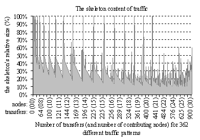
Figure 7. Proportion of the number of transfers within a skeleton, compared with the number of transfers of the corresponding traffic

6.2.Optimization - building full teams based on full teams of the skeleton

When considering the skeleton of a traffic X as another traffic, the bottlenecks of the skeleton of a traffic are the same as the bottlenecks of the traffic. Consequently, a team of a skeleton is also a team of the original traffic.

We may first obtain all full teams of the traffic’s skeleton by iteratively applying the fission algorithm on the traffic’s skeleton and by eliminating the idle categories. Then, a full team of the original traffic is obtained by adding a combination of non-congesting transfers to a team of the traffic’s skeleton.

We therefore obtain the set of a traffic’s full teams by carrying out the steps outlined in Figure 8.

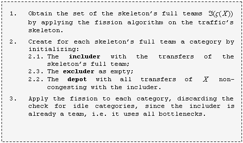
Figure 8. Optimized algorithm for retrieving all full teams of a traffic

By first applying the fission to the skeleton and then expanding the skeleton’s full teams to the traffic’s full teams, we considerably reduce the processing time.

6.3.Evaluating the reduction of the search space

Let us evaluate the reduction in search space achieved due to the search space reduction methods proposed in section 5 and in this section. We consider 23 different all-to-all traffic patterns across the network of the Swiss-T1 cluster supercomputer (see section 8). The size of the algorithm’s search space is the number of categories that are being iteratively traversed by the algorithm until all full teams are discovered.

Figure 9 shows the search space reduction for the presented four algorithms. The first one is the naïve algorithm that would build full teams only according to the coverage partitioning strategy (subsection 5.3) without considering the other optimisations. We assume that the size of the search space of the naïve algorithm is 100% and we use it as a reference for the other three algorithms. The naïve algorithm is sufficiently “smart” to avoid repetitions while exploring the full simultaneities. The second algorithm, that additionally comprises identification of blank categories (see subsection 5.4), permits, according to Figure 9, to reduce the search space to an average of 28%. The third algorithm identifies idle categories and enables at an early stage to skip evaluating all categories not leading to teams (see subsection 5.5). This third algorithm encloses all optimisations presented in section 5 and reduces the search space to an average of 20%.

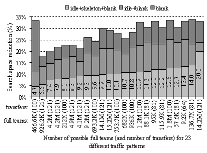
Figure 9. Search space reduction obtained by idle+skeleton+blank optimization steps

Finally the skeleton algorithm presented in this section, which according to Figure 8 is carried out in two phases, reduces the search space to an average of 10.6%. Full teams are therefore retrieved in average 9.43 times faster than in naïve algorithm of subsection 5.3, thanks to the additional three optimisation techniques, presented subsections 5.4, 5.5 and 6.2 respectively.

7. Construction of liquid schedules

In sections 5 and 6 we introduced efficient algorithms for traversing full teams of a traffic. Relying on the full team generation algorithms, this section presents methods for constructing liquid schedules for arbitrary traffic patterns on arbitrary network topologies.

7.1.Definition of liquid schedule

Let us introduce the definition of a schedule. By recalling that a partition of X is a disjoint collection of non-empty subsets of X whose union is X [Halmos74], a schedule of a traffic X is a collection of simultaneities of X partitioning the traffic X. An elements of a schedule is called time frame. The length of a schedule is the number of time frames in . A schedule of a traffic is optimal if the traffic does not have any shorter schedule. If the length of a schedule is equal to the duration of the traffic (the duration of a traffic X is the load of its bottlenecks), then the schedule is liquid. Thus a schedule of a traffic X is liquid if equation (9) holds. See also equation (2) defining the duration of a traffic X.

(9)

Figure 10 shows a liquid schedule for the collective traffic shown in Figure 4, which in turn represents an all-to-all data exchange (see Figure 3) across the network shown in Figure 2.

Figure 10. Time frames of a liquid schedule of the collective traffic shown in Figure 4

One can easily control that the timeframes of Figure 10 correspond to the following sequence , , , , , represented in form of the pictograms introduced in section 3. Recall that each pictogram in the sequence represents several transmissions that can be carried out simultaneously. For example the sequence’s second pictogram , visualizes four simultaneous transfers: to , to , to and to , wherein are the source nodes and are the destination nodes of the network of Figure 2. These four simultaneous transfers correspond to the second time frame of Figure 10: .

If a schedule is liquid, then each of its time frames must use all bottlenecks. Inversely, if all time frames of a schedule use all bottlenecks, the schedule is liquid.

The necessary and sufficient condition for the liquidity of a schedule is that all bottlenecks be used by each time frame of the schedule. Since a simultaneity of X is defined as a team of X, if it uses all bottlenecks of X, a necessary and sufficient condition for the liquidity of a schedule on X is that each time frame of be a team of X.

A liquid schedule is optimal, but the inverse is not always true, meaning that a traffic may not have a liquid schedule. An example of traffic having no liquid schedule is shown in Figure 12. This traffic is to be carried across the network shown in Figure 11. There are three bottleneck links in the network . Since there is no combination of non-congesting transfers that can simultaneously use all three bottleneck links , this traffic contains no team and therefore has no liquid schedule.

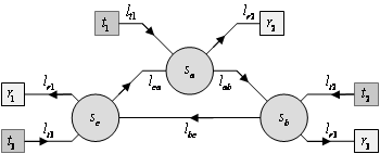
Figure 11. There exists a traffic of three transmissions across this network that has no team and therefore no liquid schedule

Figure 12. A traffic consisting of thee transmissions to be carried across the network shown in Figure 11

The rest of this section presents the liquid scheduling construction algorithm (subsection 7.2) and two optimisations (subsections 7.3 and 7.4 respectively).

In Appendix B, we show how to formulate the problem of searching for a liquid schedule with Mixed Integer Linear Programming (MILP), [CPLEX02], [Fourer03]. Appendix B presents a comparison of performances of the liquid schedule search approach presented here with that of MILP. It shows that the computation time of the MILP method is prohibitive compared with the speed of our algorithm.

7.2.Liquid schedule basic construction algorithm

In this subsection we describe the basic algorithm for constructing a liquid schedule. The basic algorithm simply consist of recursive attempts to assemble a liquid schedule out of the teams of the original traffic, until a valid liquid schedule incorporating all transfers is successfully constructed. In the following subsections (7.3 and 7.4), relying on the basic algorithm, we show how to apply further optimizations.

Our strategy for finding a liquid schedule relies on partitioning the traffic into a set of teams forming the sequence of time frames. Associate to the traffic X all its possible teams (found by the algorithm presented in section 6) which could be selected as the schedule’s first time frame. The following: is the variety of possible subtraffics remaining after the choice of the first time frame. Each of the possible subtraffics remaining after the selection of the first time frame has its own set of possibilities for the second time frame , where is a choice function. The choice of the second team for the second time frame yields a further reduced subtraffic (see Figure 13).

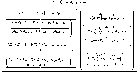
Figure 13. Liquid schedule construction tree: denotes a reduced subtraffic at the layer of the tree and denotes a candidate for the time frame ; the operator applied to a subtraffic yields the set of all possible candidates for a time frame

Dead ends are possible if there is no choice for the next time frame, i.e. no team of the original traffic may be formed from the transfers of the reduced traffic. A dead end situation may occur, for example, when the remaining subtraffic appears to be like the one shown in Figure 11 and Figure 12. Once a dead occurs, backtracking takes place.

The construction recursively advances and backtracks until a valid liquid schedule is formed. A valid liquid schedule is obtained, when the transfers remaining in the reduced traffic form one single team for the last time frame of the liquid schedule.

We rely on the construction tree of Figure 13 and assume that at any stage the choice for the next time frame is among the set of the original trafic’s teams . Thus the choice function is represented by the following equation:

(10)

In the next subsections we improve equation (10) by considering newly emerging bottlenecks at the successive time frames.

7.3.Search space reduction by considering newly emerging bottlenecks

We observe in Figure 10 that when we step from one time frame to the next, additional new bottleneck links emerge. For example from time frame 3 on, links and appear as new bottlenecks.

In the construction strategy presented in the previous subsection (7.2), according to equation (10) we consider as a possible time frame any team of the original traffic X that can be built from the transfers of the reduced subtraffic. A schedule is liquid if and only if (IFF) each time frame is not only a team of the original traffic but is also a team of the reduced subtraffic (see Appendix C for a formal proof). If is a liquid schedule on X and A is a time frame of , then is a liquid schedule on .

Thus a liquid schedule may not contain a time frame which is a team of the original traffic but is not a team of a subtraffic obtained by removing some of the previous time frames. Therefore, at each iteration, we can limit our choice on the collection of only those teams of the original traffic which are also teams of the current reduced subtraffic. Since the reduced subtraffic contains additional bottleneck links, there are less teams in the reduced subtraffic than teams remaining from the original traffic.

Therefore, in the liquid schedule construction diagram presented in Figure 13, regarding the choice function we can replace equation (10) by equation (11):

(11)

By considering in each time frame all occurring bottlenecks, with the new equation (11) we considerably speed up the construction.

7.4.Liquid schedule construction optimization by considering only full teams

In Appendix D we have shown that if a liquid schedule exists and if it can be constructed by the choice of teams, then a liquid schedule can be also constructed by limiting the choice only to full teams (see also [Gabrielyan03] and [Gabrielyan04A]).

Therefore in the construction algorithm represented by the diagram of Figure 13, the function for the choice of the teams, may be further narrowed from the set of all teams, equation (11) to the set of full teams only:

(12)

When replacing the choice function equation from (10) to (11) and then from (11) to (12) we make sure that the new equations have no impact on the solvability of the problem. The liquid schedule construction is speeded up, thanks to the reduction in choice, summarized by expressions (13) and (14) below:

(13)

and therefore also:

(14)

8. Experimental verification

In this section we present the results of application of liquid schedules to data communications carried out across a real network. In subsection 8.1 we present the network on which the experiments were carried out. We select several hundred of traffic patterns across the considered network. Measurements of aggregate communication throughputs, presented in subsection 8.2, enable us to validate the efficiency of applying liquid schedules in real networks.

8.1.Swiss-Tx cluster supercomputer and 362 test traffic patterns

The experiments are carried out across the interconnection network of the Swiss-T1 cluster supercomputer (see Figure 14). The network of Swiss-T1 forms a K-ring [Kuonen99B] and is built on TNET switches. The routing between pairs of switches is static. The throughputs of all links are identical and equal to 86MB/s. The cluster consists of 32 nodes, each one comprising 2 processors [Kuonen99A], [Gruber01], [Gruber02], [Gruber05]. The cluster thus comprises a total of 64 computing processors. Each processor has its own individual connection to the network. The network enables transmissions of large messages at low latencies. Wormhole switching is employed for this purpose.

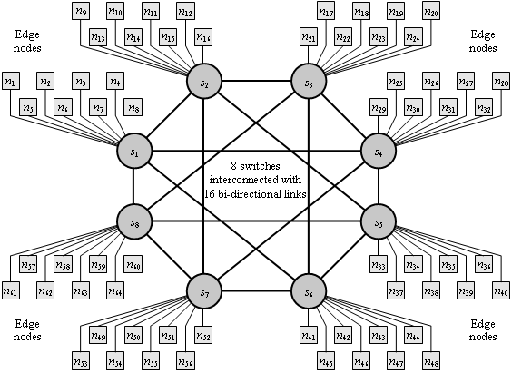
Figure 14. Architecture of the Swiss-T1 cluster supercomputer interconnected by a high performance wormhole switch fabric

Communication between a pair of any two switches requires at most one intermediate switch. The routing is summarized in Figure 15. Transmissions from switch i to switch j are routed through the switch with the number located at the position of the table. Symbol “↔” indicates that the two switches are connected by a direct link.

Text Box: Routing table
1 2 3 4 5 6 7 8
1 ↔ 2 ↔ 4 ↔ 8 ↔
2 ↔ ↔ 7 ↔ 3 ↔ 5
3 2 ↔ ↔ 4 ↔ 8 ↔
4 ↔ 7 ↔ ↔ 7 ↔ 3
5 4 ↔ 4 ↔ ↔ 6 ↔
6 ↔ 3 ↔ 7 ↔ ↔ 1
7 8 ↔ 8 ↔ 6 ↔ ↔
8 ↔ 5 ↔ 3 ↔ 1 ↔

Figure 15. The routing table of the Swiss-Tx supercomputer shown in Figure 14

We perform our experiments on a number of different data intensive traffic patterns across the network of the Swiss-T1 cluster. We limit ourselves by only those traffic patterns, where within each node one of the processors is only transmitting and the other one is only receiving. For any given allocation of nodes we have an equal number of sending and receiving processors and we assume a traffic pattern where each sending processor transmits a distinct message (of the same size) to each receiving processor. Thus, according to our assumptions, if there are n allocated nodes (i.e. pairs of processors), then there are transmissions to be carried out.

The Swiss-T1 cluster supercomputer comprises 32 nodes, 8 switches and 4 nodes per switch. We have therefore 5 possibilities of allocating nodes to each switch (from 0 to 4 nodes). This yields different node allocation patterns. To limit our choice to really different patterns of underlying topologies, we have computed the liquid throughputs for each of the 390625 topologies (taking into account the static routing). Because of various symmetries within the network, many of these topologies yield an identical liquid throughput and only 362 topologies yielding different liquid throughput values were obtained.

Figure 16 shows these 362 traffic patterns (topologies), each one being characterized by the number of contributing nodes and by its liquid throughput. Depending on how a given number of nodes are allocated in the cluster, the corresponding underlying network changes its topology considerably. Therefore for any given number of nodes, Figure 16 shows that the liquid throughput varies considerably. The management system for Computing in Distributed Networked Environment (CODINE) and the Load Sharing Facility (LSF) are the job allocation and the scheduling consoles used in Swiss-T1 [Byun00], [Hassaine02]. Taking into account the data of Figure 16 the CODINE and LSF job allocation systems of Swiss-T1 are experimentally tuned for communication intensive programs (of high priority). In these experiments the allocation strategy is simple and the fairness among several communication intensive jobs is not considered.

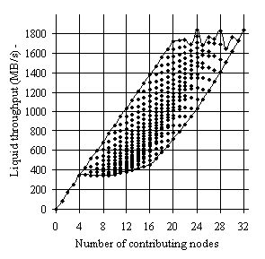
Figure 16. For a given number contributing nodes all possible allocation of nodes yielding different liquid throughputs

These 362 topologies may be also placed along one axis, sorted first by the number of nodes and then according to their liquid throughput, as shown in Figure 17.

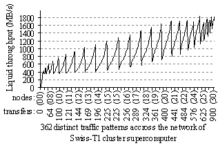
Figure 17. The 362 topologies of Figure 16 yielding different liquid throughput values placed along one axis, sorted first by the number of contributing nodes and then by their liquid throughputs

8.2.Real traffic throughout measurements

The 362 traffic patterns of Figure 16 and Figure 17 were scheduled both by our liquid scheduling algorithms and according to a topology-unaware round-robin schedule (or randomly). Overall throughput results for each method are measured and presented for comparison. In each chart, the theoretical liquid throughput values of Figure 17 are given for comparison with the measured values.

Figure 18 shows the overall communication throughput of 362 traffic patterns carried out by a topology-unaware round-robin schedule. The size of messages, i.e. the amount of data transferred from each transmitting processor to each receiving processor, is equal to 2MB. For each traffic pattern, 20 measurements were made and the chart shows the median of their throughputs (the black dots). According to the chart, the round-robin schedule yields a throughput which is far below the liquid throughput of the network. Tests with various other topology-unaware methods (such as transmission in random order or in FIFO order) yield to throughputs not which are not better than the one of the round-robin schedule.

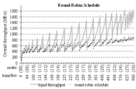
Figure 18. Theoretical liquid throughput and measured round-robin schedule throughput for 362 network sub topologies.

Then, we carried out the same 362 traffic patterns but scheduled according to the liquid schedules found by our algorithms. The overall throughput results are shown in Figure 19. The size of the messages (processor to processor transfers) is of 5MB (even larger than for the measurements of Figure 18). Each black dot represents the median of 7 measurements. The chart shows, that the measured aggregate throughputs (black dots) are very close to the theoretically expected values of the liquid throughput (gray curve).

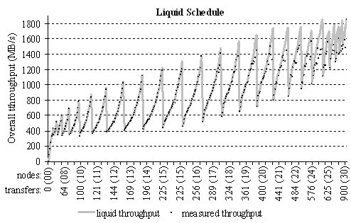
Figure 19. Predicted liquid throughput and measured throughput according to the computed liquid schedule

Comparison of the chart of Figure 18 with that of Figure 19 demonstrates that for many traffic patterns, liquid scheduling allows to increase the aggregate throughput by a factor of two compared with topology-unaware round-robin scheduling. The gain is especially significant for large topologies and heavy traffics.

Thanks to the full team space reduction algorithms (sections 5 and 6) and liquid schedule construction optimizations (section 7), the computation time of a liquid schedule for more than 97% of the considered topologies takes no more than 1/10 of a second on a single PC.

9. Conclusions

In circuit-switching coarse-grained congestion prone networks (e.g. optical lightpath routing and wormhole switching), significant throughput losses occur due to attempts to simultaneously carry out transfers sharing common communication resources. The communications must be scheduled such that congesting transmissions are not carried our simultaneously. We proposed a liquid scheduling algorithm, which properly schedules the transmissions within the time as short as the utilization time of a bottleneck link. A liquid schedule yields therefore an aggregate throughput equal to the network’s theoretical upper limit, i.e. its liquid throughput. To construct a liquid schedule, we must chose time frames utilizing all bottleneck links and incorporating as many transfers as possible.

These saturated subsets of non-congesting transfers using all bottleneck links are called full teams and are needed for the construction of a liquid schedule. An efficient construction of liquid schedules relies on the fast retrieval of full teams. We obtained a significant speed up in the construction algorithm by carrying out optimizations in the retrieval of full teams and in their further assembling into a schedule. The liquid schedule construction algorithm and its optimizations are briefly outlined below.

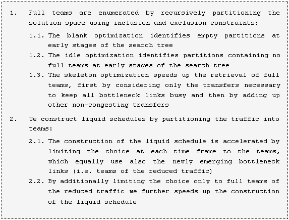
Figure 20. Liquid schedule construction and the relevant optimizations

Measurements on the traffic carried out on various sub-topologies of the Swiss-T1 cluster supercomputer have shown that for most of the sub-topologies we are able to increase the overall communication throughput by a factor between 1.5 and 2 (see Figure 21).

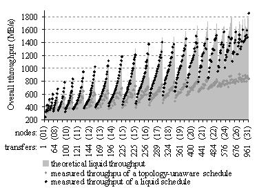
Figure 21. The overall throughputs of hundreds of different traffic patterns carried out according a liquid schedule and according a topology unaware schedule, comparison with a theoretical upper limit

In congestion prone coarse-grain transmission networks, liquid scheduling considerably improves the overall throughput by ensuring optimal utilization of transmission resources (e.g. the bottleneck communication links, wavelengths and time frames). By avoiding contentions, liquid schedules minimize the overall transmission time of large communication patterns containing many congesting transfers.

Appendix A. Congestion graph coloring heuristic approach

The search for a liquid schedule requires the partitioning of the traffic into sets of mutually non-congesting transfers. This problem can be also represented as the problem of the conflict graph coloring [Beauquier97]. Vertices of the conflict (or congestion) graph represent the transfers. Edges between vertices represent congestions between the transfers.

Figure 22 shows a congestion graph that corresponds to the all-to-all traffic pattern across the network of Figure 2, which consists of 25 transfers. These transfers are shown in Figure 3 in form of pictograms and in Figure 4 in form of sets of communication links. The vertices of the congestion graph are labeled with two indexes , such that vertex represents the transfer from the sending node i to the receiving node j. Vertex , for example represents the transfer from node to node , denoted as in Figure 3 and as in Figure 4.

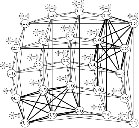
Figure 22. Congestion graph corresponding to the traffic pattern of Figure 3 across the network of Figure 2: the vertices of the graph represent the 25 transfers, the edges represent congestions between the transfers

An edge between two vertices occurs due to one or more links shared between two corresponding transfers. Therefore each edge of the congestion graph can be labeled by the link(s) causing the congestion. In Figure 22 we marked in bold the edges occurred due to the bottleneck links and (see the concerned network diagram in Figure 2). The 15 bold edges between any two of the following vertices (1,4), (1,5), (2,4), (2,5), (3,4), (3,5) represent the congestions due to the bottleneck link . The other 15 bold edges between the vertices (4,1), (4,2), (4,3), (5,1), (5,2), (5,3) represent the congestions due to the bottleneck link .

According to the graph coloring problem, the vertices of the graph must be colored such that no two vertices have the same color if they are connected. The objective of the graph coloring problem is to properly color the graph using a minimal number of colors. The graph coloring is an NP-complete problem, but various heuristic algorithms exist.

Once the graph is properly colored, vertices having the same color can represent a time frame of the liquid schedule, since the corresponding transfers can be carried out simultaneously without congestions. Whenever a liquid schedule exists, an optimal solution of the graph coloring problem corresponds to a liquid schedule and the chromatic number of the graph’s optimal coloring is therefore the length of the liquid schedule. A heuristic graph coloring algorithm however may find solutions requiring several more colors, reducing therefore the throughput of the corresponding schedule.

Congestion graphs corresponding to traffic patterns carried out across the network of Swiss-T1 cluster supercomputer have relatively low density of edges (see Figure 23). For example, an all-to-all data exchange on the Swiss T1 cluster with 32 transmitting and 32 receiving processors results in a graph with vertices and 48704 edges (the corresponding complete graph has 523776 edges that is eleven times more).

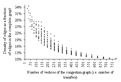
Figure 23. Number of edges in the 362 congestion graphs corresponding to the traffic patterns of Figure 16 and Figure 17

We compared our method of finding a liquid schedule with the results obtained by applying a fast greedy graph coloring algorithm Dsatur [Brelaz79], [Culberson97], which carries out the steps shown in Figure 24.

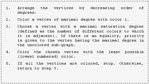
Figure 24. Dsatur graph coloring heuristic algorithm

Although the greedy algorithm is fast, often it induces additional colors. Figure 25 shows the loss of performance for 362 traffic patterns of Figure 16 and Figure 17 across the network of Swiss-T1 cluster supercomputer (see Figure 14 and Figure 15). The throughput loss of the greedy algorithm is compared with the liquid schedule algorithm. The losses occur due to the additional unnecessary colors induced by the greedy graph coloring algorithm.

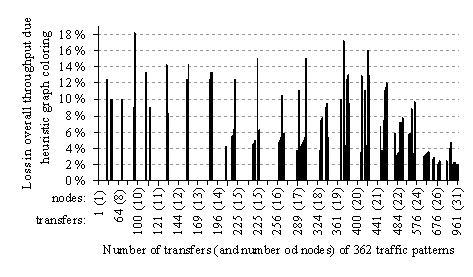
Figure 25. Loss in throughput induced by schedules computed with the Dsatur heuristic algorithm

For 74% of the topologies there is no loss of performance. For 18% of the topologies, the performance loss is below 10% and for 8% of the topologies, the loss of performance is between 10% and 19%.

The computation time of the greedy algorithm is polynomial and compares therefore favorably with the algorithm searching for the liquid schedule. However, for large data exchanges, the cost of the liquid scheduling algorithm, not exceeding most of the time 1/10 of a second (see Appendix B), is negligible compared with the gain in communication time yielding from liquid schedules.

The liquid scheduling algorithm can be regarded as an efficient congestion graph coloring algorithm. However, liquid scheduling algorithm cannot be however applied to the general problem of graph coloring, since the liquid scheduling algorithm relies on the fact that the transfers (the vertices of the abstracted graph), are in fact sets consisting of communication links. For example the algorithm for searching the full teams of a traffic, relies on the search of the full teams of the traffic’s skeleton (see subsection 6.2), which in turn relies on transfers using the bottleneck links.

Appendix B. Comparison of liquid scheduling algorithm with Mixed Integer Linear Programming

The problem of liquid scheduling can be formulated and solved with Mixed Integer Linear Programming (MILP), see [CPLEX02], [Fourer03]. The problem of minimizing of the number of timeframes (and/or wavelengths) can be represented as an MILP objective.

We represent the network as a directed graph . The routing is represented by a parameter , indexed above by the source and destination nodes (, ) and below by the network link . This parameter indicates if the transmission (flit stream flow for wormhole switching or lightpaths for optical networks) from the source s to the destination d traverses the link e. It is set to 1 if the transmission uses the link e and to 0 otherwise.

(15)

Given is also the traffic pattern X comprising pairs of communication nodes . The transmissions of the traffic pattern are allocated to timeframes according to the variable . The variable is 1 if the transmission is allocated to the timeframe t and is 0 otherwise.

(16)

The objective is to allocate the transfers such that the number T is minimized. We may formulate this as follows:

Minimize: T

subject to:

(17)

and

(18)

Relation (17) represents the simultaneity constraint: number of transfers in a timeframe using a given network link can be either 0 or 1. Equation (18) represents the partitioning constraint. The traffic X is partitioned into time frames of a schedule, therefore each transfer of the traffic must be assigned to one and only one time slot.

The present problem is hard to solve with MILP. For the 362 test bed topologies introduced in subsection 8.1 (see Figure 16 and Figure 17), we compared Mixed Integer Linear Programming (MILP) method with liquid scheduling algorithm. The computation speed of MILP is far below that of our liquid scheduling algorithm (Figure 26). Our algorithm is on average about 4000 times faster than MILP.

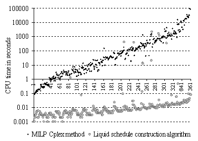
Figure 26. Running times for computing liquid schedules by MILP Cplex method and by liquid schedule construction algorithm

Appendix C. Assembling a liquid schedule: Considering teams of the reduced traffic instead of the teams of the original traffic

The basic algorithm for construction of liquid schedules (see subsection 7.2) assumes that a liquid schedule can be assembled by considering various combinations of teams of the original traffic. For example if a certain combination of teams of X is already selected (from the set of all teams of X) and there still remains a subtraffic of not yet carried out (scheduled) transfers, then, according to the basic algorithm, the following teams of the original traffic must be considered in the choice of the next timeframe. See subsection 7.2, equation (10) and Figure 13.

The two theorems prove that we can restrict our choice of possibilities when selecting successive time frames without affecting the solvability.

Theorem 1 shows that by removing a time frame (i.e. a team) from a liquid schedule, we form a new liquid schedule on the remaining traffic. The remaining traffic may have additional bottlenecks. For example, in Figure 10, from time frame 3 on, links and appear as additional bottlenecks, from time frame 5 on, the links and also appear as additional bottlenecks (making the total number of bottlenecks equal to 6).

Additionally emerged bottlenecks allow us to limit our choice of a timeframe from a large set of teams of the original traffic to a smaller set of teams of the reduced traffic. According to theorem 2, this does not affect the solvability. The statement appears logically clear (in terms of the remaining transmissions to be carried out). The exercise of giving a formal proof is provided for the sake of keeping the mathematical model complete.

Theorem 1. Let be a liquid schedule on X and A be a time frame of . Then is a liquid schedule on .

Proof. By definition schedule is liquid if its length is equal to the duration of the traffic (equation (9) of subsection 7.1). Clearly A is a team of X. Remove the team A from X so as to form a new traffic . The duration of the new traffic is the load of the bottlenecks in .

The load of bottlenecks of X in X is the highest and therefore is more than the load of all other links at least by 1. By removing a team of X the load of all bottleneck links is reduced by 1. Therefore, a link which is bottleneck in X is still a bottleneck in . Thus the bottlenecks of include the bottlenecks of X.

The load of a bottleneck of X is decreased by one in the new traffic and therefore the duration of is the duration of X decreased by one, i.e. . The schedule without the element A is a schedule for by definition of a schedule given in subsection 7.1 (a schedule is a collection of simultaneities partitioning the traffic). Obviously . Therefore the new schedule has as many time frames as the duration of the new traffic is. Hence is a liquid schedule on . ■

In other words, if the traffic has a liquid schedule, then a schedule reduced by one team is a liquid schedule on the reduced traffic. The repeated application of Theorem 1 implies that any non-empty subset of a liquid schedule is a liquid schedule on the correspondingly reduced traffic.

Theorem 2. If, by traversing each team A of a traffic X none of the sub-traffics has a liquid schedule, then the traffic X does not have a liquid schedule either.

Proof. Let us suppose that X has a liquid schedule . Then a time frame A of shall be a team of X. Further, according to Theorem 1, the schedule shall be a liquid schedule for . Therefore for at least one team A of X the sub-traffic has a liquid schedule. This proves the theorem by contraposition. ■

Theorem 2 implies that if X has a liquid schedule, at least one team A of X will be found, such that the sub-traffic has a liquid schedule . Obviously will be a liquid schedule for X.

Instead of considering for the set of possible time frames all teams of the original traffic included in the current sub-traffic , i.e. , we propose to consider for the set of possible time frames (at the current node of the construction tree) all teams of the current sub-traffic, i.e. .

By induction, theorem 2 implies that If a solution for X (i.e. a liquid schedule on X) exists, then this algorithm will necessarily find it.

Since the teams of the current sub-traffic together with the bottlenecks of the original traffic X must also use the additional bottlenecks of , the number of teams of the current subtraffic is smaller or equal to the number of teams of the original traffic whose transfers belong to the current subtraffic:

(19)

Therefore less possible teams need to be considered when building the schedule. The solution space is not affected, since theorem 2 is valid at any level of the search tree.

The construction algorithm traverses the tree in depth-wise order (Figure 13). A solution is found when the current node (sub-traffic) forms a single team. The path from the root to that leaf node forms the set of teams yielding the liquid schedule. The example of a liquid schedule of Figure 10 shows that each timeframe incorporates additionally also the bottlenecks (marked in bold) of the remaining reduced traffic. Therefore each timeframe is also a team of the reduced traffic. A node, in the construction tree, is a dead end if the corresponding sub-traffic does not have a team (see for example Figure 11 and Figure 12). In that case the algorithm backtracks and evaluates other choices. Evaluation of all choices ultimately leads to a solution if it exists.

Appendix D. Assembling a liquid schedule: Considering full teams of the reduced traffic instead of all its teams

Assuming the liquid schedule construction algorithm of subsection 7.3, we can build a liquid schedule by further limiting the choice of teams of the reduced subtraffic to its full teams.

Let us modify a given liquid schedule so as to convert one of its teams into a full team. Let a traffic X have a liquid schedule . Let A be a time frame of . If A is not a full team of X, then, by moving the necessary transfers from other time frames of , we can convert the team A into a full team. Evidently, by doing so, the properties of liquidity (partitioning, simultaneousness and length) of are not affected. Therefore if X has a solution then it has also a solution when any one of its selected time frames is full.

Therefore if a liquid schedule is possible to built, then it can be built by a choice of a full team A of the current reduced traffic . Therefore the choice of the teams in the construction tree of Figure 13 may be narrowed from the set of all teams to the set of full teams only, i.e. . The optimization of subsection 7.4 relies on this (see equations (12), (13) and (14)). An efficient algorithm for retrieving the set of all full teams is presented in Figure 8.

Figure 10 shows a liquid schedule constructed with full teams. For any given timeframe, all transfers of all successive timeframes are congesting with that timeframe.

References

[Ayad97] N.M.A. Ayad, F.A. Mohamed, “Performance analysis of a cut-through vs. packet-switching techniques”, 2nd IEEE Symposium on Computers and Communications, 1-3 July 1997, pp. 230-234

[Beauquier97] B. Beauquier, J.C. Bermond, L. Gargano, P. Hell, S. Pérennes, U. Vaccaro, “Graph Problems Arising from Wavelength-Routing in All-Optical Networks”, IPPS’97: WOCS’97 - 2nd IEEE Workshop on Optics and Computer Science, April 1997

[Bermond96] J.-C. Bermond, L. Gargano, S. Perennes, A. A. Rescigno, and U. Vaccaro, “Efficient collective communication in optical networks”, ICALP’96 - Lecture Notes in Computer Science 1099, Springer Verlag, Berlin 1996, pp. 574-585

[Boden95] N.J. Boden, D. Cohen, R.E. Felderman, A.E. Kulawik, C.L. Seitz, J.N. Seizovic, Wen-King Su, “Myrinet: a gigabit per second local area network,” IEEE Micro, February 1995, vol. 15, issue 1, pp. 29-36

[Brauss99B] Stephan Brauss, “Communication Libraries for the Swiss-Tx Machines”, EPFL Supercomputing Review, Nov 1999, pp. 12-15, http://sawww.epfl.ch/SIC/SA/publications/SCR99/scr11-page12.html

[Brelaz79] Daniel Brelaz, “New Methods to Color the Vertices of a Graph”, Communication of the ACM, April 1979, Vol. 22, Issue 4, pp. 251-256

[Byun00] Chansup Byun, Christopher Duncan, “A Comparison of Job Management Systems in Supporting HPC ClusterTools”, SUPerG, Vancouver, Fall 2000, http://www.indiana.edu/~uits/rac/mgmt.pdf

[Caragiannis02] I. Caragiannis, Ch. Kaklamanis, P. Persiano, “Wavelength Routing in All-Optical Tree Networks: A Survey”, Bulletin of the European Association for Theoretical Computer Science, 2002, Vol. 76, pp. 104-112

[CERN04] Large Hadron Collider, Computer Grid project, CERN, 2004, http://lcg.web.cern.ch/LCG/

[Chan01] S.-H.Gary Chan, “Operation and cost optimization of a distributed server architecture for on-demand video services”, IEEE Communications Letters, September 2001, Vol. 5, Issue 9, pp. 384-386

[Chiu89] Dah-Ming Chiu, Raj Jain, “Analysis of the increase and decrease algorithms for congestion avoidance in computer networks”, Computer Networks and ISDN Systems, 1989, Vol. 17, pp. 1-14

[Colajanni99] M. Colajanni, B. Ciciani, F. Quaglia, “Performance Analysis of Wormhole Switching with Adaptive Routing in a Two-Dimensional Torus”, Euro-Par’99, Toulose, France, Spinger-Verlang, August – September, 1999

[CPLEX02] ILOG CPLEX 8.0, User's Manual, ILOG SA, Gentilly, France, 2002

[Culberson97] Joseph Culberson, “Graph Coloring Programs Manual”, University of Alberta, Canada, 1997, http://www.cs.ualberta.ca/~joe/Coloring/Colorsrc/manual.html

[Duato99] J. Duato, A. Robles, F. Silla, R. Beivide, “A comparison of router architectures for virtual cut-through and wormhole switching in a NOW environment”, SPDP’99 - IEEE Symposium on Parallel and Distributed Processing, 12-16 April 1999, pp. 240-247

[Dvorak05] Vaclav Dvorak, “Scheduling Collective Communications on Wormhole Fat Cubes”, 17th International Symposium on Computer Architecture and High Performance Computing, 24-27 Oct 2005, pp. 27-34

[EWSD04] Siemens Carrier Networks, EWSD Digital Switching System, April 2004, http://www.icn.siemens.com/carrier/products/switching/ewsdsw.html

[Fourer03] R. Fourer, D. M. Gay, B. W. Kernighan, AMPL: A Modeling Language for Mathematical Programming, Thomson Learning Brooks/Cole, 2003

[Gabrielyan03] Emin Gabrielyan, Roger D. Hersch, “Network Topology Aware Scheduling of Collective Communications”, ICT’03 - 10th International Conference on Telecommunications, 2003, pp. 1051-1058

[Gabrielyan04A] Emin Gabrielyan, Roger D. Hersch, “Liquid Schedule Searching Strategies for the Optimization of Collective Network Communications”, 18th International Multi-Conference in Computer Science & Computer Engineering: PCC’04 - Pervasive Computing and Communications, Las Vegas, USA, 21-24 June 2004, CSREA Press, vol. 2, pp. 834-848

[Gruber01] Ralf Gruber, Pieter Volgers, Alessandro De Vita, Massimiliano Stengel, “Commodity computing results from the Swiss-Tx project”, Electronic Notes in Future Generation Computer Systems, 2001, Vol. 1

[Gruber02] Ralf Gruber, Alessandro de Vita, Massimiliano Stengel, Trach-Minh Tran, “Application Dedicated Clustering”, EPFL Supercomputing Review, May 2002, pp. 37-40, http://sawww.epfl.ch/SIC/SA/SPIP/Publications/IMG/pdf/scr13_page37.pdf

[Gruber05] Ralf Gruber, “High Performance Computing Methods”, Swiss-Tx and Swiss Grid, 2005, http://pleiades.epfl.ch/~rgruber/cours/C5_6part1.0.ppt

[H323] H.323 Standards, http://www.openh323.org/standards.html

[Halmos74] Paul R. Halmos, Naive Set Theory, Springer-Verlag New York Inc, 1974, pp. 26-29

[Hassaine02] Omar Hassaine, “HPC Administration Tips and Techniques”, CPR Engineering-HPC, Sun BluePrints OnLine, October 2002, http://www.sun.com/blueprints/1002/817-0079-10.pdf

[Horst95] R. Horst, “TNet: A Reliable System Area Network”, IEEE Micro, February 1995, vol. 15, Issue 1, pp. 37-45

[InfiniBand] InfiniBand Trade Association, http://www.infinibandta.org/

[Jagannathan02] S. Jagannathan, A. Tohmaz, A Chronopoulos, H.G. Cheung, “Adaptive admission control of multimedia traffic in high-speed networks”, IEEE International Symposium on Intelligent Control, 27-30 Oct 2002, pp. 728-733

[Kartalopoulos00] Stamatios V. Kartalopoulos, “What is WDM technology”, Technology and Trends for International Optical Engineering Community, November 2000, http://www.spie.org/web/oer/november/nov00/wdm.html

[Kuonen99A] Pierre Kuonen, Ralf Gruber, “Parallel computer architectures for commodity computing and the Swiss-T1 machine”, EPFL Supercomputing Review, Nov 1999, pp. 3-11, http://sawww.epfl.ch/SIC/SA/publications/SCR99/scr11-page3.html

[Kuonen99B] Pierre Kuonen, “The K-Ring: a versatile model for the design of MIMD computer topology”, HPC’99 - High-Performance Computing Conference, San Diego, USA, April 1999, pp. 381-385

[Liu01] Pangfeng Liu, Jan-Jan Wu, Yi-Fang Lin, Shih-Hsien Yeh, “A simple incremental network topology for wormhole switch-based networks”, 15th International Parallel and Distributed Processing Symposium, 23-27 April 2001, pp. 6-12

[Loh96] P.K.K. Loh, Wen Jing Hsu, Cai Wentong, N. Sriskanthan, “How network topology affects dynamic loading balancing”, Parallel & Distributed Technology: Systems & Applications, Fall 1996, Vol. 4, Issue 3, pp. 25-35

[Maach04] Abdelilah Maach, Gregor v. Bochmann, Hussein Mouftah, “Contention avoidance in optical burst switching”, ICN’04 - International Conference on Networking, 2004, pp. 1-7

[Mandjes02] M. Mandjes, D. Mitra, W. Scheinhardt, “Simple models of network access, with applications to the design of joint rate and admission control”, INFOCOM’02, 23-27 June 2002, Vol. 1, pp. 3-12

[Melamed00] Benjamin Melamed, Khosrow Sohraby, Yorai Wardi, “Measurement-Based Hybrid Fluid-Flow Models for Fast Multi-Scale Simulation”, DARPA/NMS Project, Sep 2000, http://204.194.72.101/pub/nms2000sep/UMissouri-KC.pdf

[Naghshineh93] M. Naghshineh, R. Guerin, “Fixed versus variable packet sizes in fast packet-switched networks”, INFOCOM’93, March 28 - April 1, 1993, vol. 1, pp. 217-226

[Petrini01] Fabrizio Petrini, Adolfy Hoisie, Wu-chun Fengy, Richard Grahamy, “Performance Evaluation of the Quadrics Interconnection Network”, 15th International Parallel and Distributed Processing Symposium, 23-27 April 2001, pp. 1698-1706

[Petrini03] Fabrizio Petrini, Adolfy Hoisie, Wu-chun Fengy, Richard Grahamy, Salvador Coll , Eitan Frachtenberg, “Performance Evaluation of the Quadrics Interconnection Network”, Cluster Computing 6, 2003, pp. 125-142

[Qiao99] Chunming Qiao, Myungsik Yoo, “Optical Burst Switching (OBS) - A New Paradigm for an Optical Internet”, Journal of High Speed Networks, 1999, vol. 8, no. 1, pp. 69-84

[Quadrics] www.quadrics.com

[Ramaswami97] R. Ramaswami, G. Sasaki, “Multiwavelength optical networks with limited wavelength conversion”, INFOCOM’97, 7-11 April 1997, vol. 2, pp. 489-498

[Rexford96] Jennifer Rexford, Kang G. Shin, “Analytical Modeling of Routing Algorithms in Virtual Cut-Through Networks”, University of Michigan, 1996

[Shin96] K.G. Shin, S.W. Daniel, “Analysis and implementation of hybrid switching”, IEEE Transactions on Computers, June 1996, Vol. 45, Issue 6, pp. 684-692

[SIP] SIP Forum, http://www.sipforum.org/

[Sitaram00] Dinkar Sitaram, Asit Dan, “Multimedia Servers”, Morgan Kaufmann Publishers, San Francisco California, 2000, pp. 69-73

[Steen05] Aad J. van der Steen, Jack J. Dongarra, “Infiniband” from the “Overview of Recent Supercomputers”, http://www.phys.uu.nl/~steen/web05a/infiniband.html

[Stern99] Thomas E. Stern, Krishna Bala, “Multiwavelength Optical Networks: A Layered Approach”, Addison-Wesley, May 1999

[Turner99] Jonathan Turner, “Terabit Burst Switching”, Journal of High Speed Networks, 1999, vol. 8, no. 1, pp. 3-16

[Turner02] Jonathan Turner, “Terabit Burst Switching Progress Report”, Washington University in St. Louis, 14 May 2002

[Yocum97] K.G. Yocum, J.S. Chase, A.J. Gallatin, A.R. Lebeck, “Cut-through delivery in Trapeze: An Exercise in Low-Latency Messaging”, 6th International Symposium on High Performance Distributed Computing, 5-8 August 1997, pp. 243-252

Glossary

3G 3rd Generation mobile communication

3GPP 3rd Generation Partnership Project

ADIO Abstract Device Interface for Portable Parallel I/O

ADSL Asynchronous Digital Subscriber Line

AMPL A Mathematical Programming Language

AMR Adaptive Multi-Rate voice codec 4.75 - 12.2 kbps

ANL Argonne National Laboratory, http://www.anl.gov/

API Application Program Interface

ARPANET Advanced Research Projects Agency Network

ARQ Automatic Repeat request

ATM Asynchronous Transfer Mode, a telecommunication protocol

BER Bit Error Rate

CODINE / GRD Computing in Distributed Networked Environment / Global Resource Director

CPLEX A high-performance linear programming solver

CPU Central Processing Unit

CTI Swiss Commission for Technology and Innovation

DER Decoding Error Rate

DMA Direct Memory Access

DoD The U.S. Department of Defense

DoS Deny of Service

DWDM Dense Wavelength Division Multiplexing

E/O Electro/Optical conversion

EIGRP Enhanced Interior Gateway Routing Protocol

EPFL École Polytechnique Fédérale de Lausanne, Swiss Federal Institute of Technology Lausanne, http://www.epfl.ch/

ETHZ Eldgenössische Technische Hochschule Zürich, Swiss Federal Institute of Technology Zurich

FCI Fast Communication Interface

FEC Forward Error Correction

FIFO First In, First Out

flit Flow unit, in wormhole and cut-through switching

g723r53 High complexity voice codec G.723.1 5300 bps

g723r63 High complexity voice codec G.723.1 6300 bps

g729r8 Low complexity voice codec G.729 8000 bps

GPS Global Positioning System

gsmfr High complexity voice codec GSMFR 13200 bps

HPC High Performance Computing

HTTP HyperText Transfer Protocol

I/O Input-Output

IFF If and only if

ILOG Developer and distributor of linear programming solutions, http://www.ilog.com

IMP Interface Message Processor

IOS Internet Operating System

IP Internet Protocol

ISP Internet Service Provider

ITSP Internet Telephony Service Provider

ITU International Telecommunication Union

ITU-T International Telecommunication Union-Telecommunication Standardization Sector

LAN Local Area Network

LP Linear Programming

LSF Load Sharing Facility, a scheduling system in HPC

LSP Laboratoire de Systèmes Périphériques, Peripheral Systems Laboratory of EPFL, http://lsp.epfl.ch

LT Luby Transform Code

MANET Mobile Ad-hoc Network

MBMS Multimedia Broadcast/Multicast Service

MDS Maximum Distance Separable

MEMS Micro-Electro-Mechanical Systems

MILP Mixed Integer Linear Programming

MPEG Moving Picture Experts Group

MPI Message Passing Interface

MPICH “CH” in MPICH stands for “Chameleon”, symbol of adaptability to one’s environment and thus of portability

MYRINET is a high-speed local area networking system designed by Myricom to be used as an interconnect between multiple machines to form computer clusters

NAT Network Address Translation

NP-complete Non-deterministic Polynomial time

O/E Optical/Electrical conversion

O/E/O Optical/Electrical/Optical conversion

OADM Optical Add/Drop Multiplexer

OBS Optical Burst Switching

OLT Optical Line Terminal

ORNL Oak Ridge National Laboratory, http://www.ornl.gov/

OS Operating System

OXC Optical Cross-Connect

PBS Portable Batch System, a scheduling system in HPC

QoS Quality of Service

ROR Redundancy Overall Requirement

RS Reed-Solomon

RTP Real-time Transport Protocol

RTT Round Trip Time

SAN Storage Area Networks

SCS Supercomputing Systems

SFIO Striped File I/O

SIP Service Initiating Protocol

SNL Sandia National Laboratories, http://www.sandia.gov/

SONET Synchronous Optical Network

SRI Stanford Research Institute

TCP Transmission Control Protocol

TDM Time-Division Multiplexing, a technology in circuit-switched digital telephony

TNET High-performance switch-based communication network aiming at low-latency and high-bandwidth

UA User Agent

UCLA University of California, Los Angeles

UDP User Datagram Protocol

UNIX Uniplexed Information and Computing System (it was originally spelled “Unics”)

VCT Virtual Cut-Through

VOIP Voice Over IP

VPN Virtual Private Network

WAN Wide Area Network

WAP Wavelength Assignment Problem

WDM Wavelength Division Multiplexing

WIXC Wavelength-Interchanging Cross-Connect

WSXC Wavelength-Selective Cross-Connect

X.25 an ITU-T protocol standard for WAN communications that defines how connections between user devices and network devices are established and maintained

XOR Exclusive OR

Table of figures

Figure 1. Wavelength routing in optical layer 7

Figure 2. A simple network sample. 9

Figure 3. The pictograms representing the 25 transfers from all sending nodes to all receiving nodes of the network of Figure 2 10

Figure 4. Example of a traffic comprising 25 transfers carried out over the network shown in Figure 2 12

Figure 5. An initial category before fission, where symbol , represents any transfer that is in congestion with and symbol represents any transfer which is simultaneous with . 15

Figure 6. Fission of the category of Figure 5 into its positive and negative sub categories. 15

Figure 7. Proportion of the number of transfers within a skeleton, compared with the number of transfers of the corresponding traffic. 17

Figure 8. Optimized algorithm for retrieving all full teams of a traffic. 18

Figure 9. Search space reduction obtained by idle+skeleton+blank optimization steps. 19

Figure 10. Time frames of a liquid schedule of the collective traffic shown in Figure 4. 20

Figure 11. There exists a traffic of three transmissions across this network that has no team and therefore no liquid schedule 21

Figure 12. A traffic consisting of thee transmissions to be carried across the network shown in Figure 11 21

Figure 14. Architecture of the Swiss-T1 cluster supercomputer interconnected by a high performance wormhole switch fabric 25

Figure 15. The routing table of the Swiss-Tx supercomputer shown in Figure 14. 25

Figure 16. For a given number contributing nodes all possible allocation of nodes yielding different liquid throughputs 27

Figure 17. The 362 topologies of Figure 16 yielding different liquid throughput values placed along one axis, sorted first by the number of contributing nodes and then by their liquid throughputs. 27

Figure 18. Theoretical liquid throughput and measured round-robin schedule throughput for 362 network sub topologies. 28

Figure 19. Predicted liquid throughput and measured throughput according to the computed liquid schedule 29

Figure 20. Liquid schedule construction and the relevant optimizations. 30

Figure 23. Number of edges in the 362 congestion graphs corresponding to the traffic patterns of Figure 16 and Figure 17 33

Figure 24. Dsatur graph coloring heuristic algorithm.. 34

Figure 25. Loss in throughput induced by schedules computed with the Dsatur heuristic algorithm 34

Figure 26. Running times for computing liquid schedules by MILP Cplex method and by liquid schedule construction algorithm 36

Workshops and papers on Liquid Scheduling problem

- Emin Gabrielyan, “Network Topology-aware Traffic Scheduling”, 6th SOS Workshop on Distributed Supercomputing: Data Intensive Computing, 5 March 2002, Leukerbad, Switzerland [ch], [us]

- Emin Gabrielyan, Roger D. Hersch, “Network Topology Aware Scheduling of Collective Communications”, ICT’03 - 10th International Conference on Telecommunications, Tahiti, French Polynesia, 23 February - 1 March 2003, pp. 1051-1058 (ISBN 0-7803-7661-7, IEEE 03EX628, Congress 2002113141) [ch], [us]

- Emin Gabrielyan, Roger D. Hersch, “Liquid Schedule Searching Strategies for the Optimization of Collective Network Communications”, 18th International Multi-Conference in Computer Science & Computer Engineering: PCC’04 - Pervasive Computing and Communications, Las Vegas, USA, 21-24 June 2004, vol. 2, pp. 834-848 (CSREA Press, ISBN 1-932415-39-4, Set ISBN 1-932415-40-8) [ch], [us]

- Emin Gabrielyan, Roger D. Hersch, “Efficient Liquid Schedule Search Strategies for Collective Communications”, ICON’04 - 12th IEEE International Conference on Networks, Hilton, Singapore, 16-19 November 2004, vol. 2, pp 760-766 [ch], [us]

Links and printable formats

- Workshops and papers on liquid scheduling problem [CH], [US]

- Location of this page [CH], [US]

- Document format [DOC], [PDF], [HTM]

- The source files of the figures used in the document [Index]

* * *