Computing the needed redundancy overhead
of an erasure resilient code for a successful media transmission over a network
with random packet loss probability
Emin Gabrielyan
EPFL / Switzernet
emin.gabrielyan@{epfl.ch, switzernet.com}
2005-10-27
Table of contents:
III. Fast computation of
Binomial Distribution
Abstract: Packetized communications over internet behave like erasure channels. For example, files or real-time media sent over the internet are chopped into packets, and each packet is either received without error or not received. Assuming Maximum Distance Separable (MDS) erasure resilient codes; we present a method for computing the codeword overhead (needed for a satisfactory transmission) as a function from the random loss probability in the network.
I.
Secure
Media Streaming
Assuming an erasure channel and Maximum Distance Separable (MDS) systematic codes (such as Reed Solomon codes, or see an erasure resilient checksum code example) given is the following problem:
-
We are streaming an on-line media from a sender to the
receiver over a network with a packet’s random loss probability p
- In order to compensate p percent of network losses, the sender, after every M transmitted media packets, is adding some redundant packets relative to these last M packets. Since the encoder is systematic and is using MDS codes, the receiver can restore the initial media if any of M packets out of all transmitted packets are survived (out of M media packets together with their redundant packets)
- Since we are dealing with on-line media (such as a VOIP phone conversation), M cannot be infinitely large
-
Mean of the number of lost packets at the receiver for
a block of N transmitted packets is ![]() , but with random loss pattern, the probability of receiving
less than
, but with random loss pattern, the probability of receiving
less than ![]() packets can not be
neglected
packets can not be
neglected
-
Let ![]() be the number of
packets in the block containing M
media packets and
be the number of
packets in the block containing M
media packets and ![]() redundancy packets. Let the desired probability of
unsuccessful decoding at the receiver be DER (Decoding Error Rate)
redundancy packets. Let the desired probability of
unsuccessful decoding at the receiver be DER (Decoding Error Rate)
By sufficiently increasing the N, for a given M and p we can reduce the probability of
decoding failure to any desired rate. Our question is, which is the smallest N for a given ![]() that keeps the
decoding failure probability at the receiver below a given DER.
that keeps the
decoding failure probability at the receiver below a given DER.
II.
Binomial
Distribution
The probability of having n erasures in a block of N packets with a random loss probability p is known as binomial distribution and denoted as:
![]()
where ![]()
and ![]()
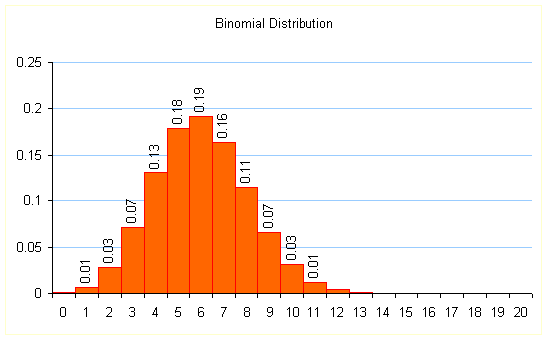
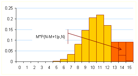
The above plot shows the distribution of n erasures out of ![]() packets with
packets with ![]()
The probability of having less than M survived packets in a block of N packets is the probability of having ![]() or more erasures; it is
computed and denoted as follows:
or more erasures; it is
computed and denoted as follows:
![]()
For a given M and p, with increase of N this probability decreases. Assume M is 5 and ![]() . The below plot shows four Binomial distributions for a
value of N starting from 9 and
enlarging up to 15.
. The below plot shows four Binomial distributions for a
value of N starting from 9 and
enlarging up to 15.
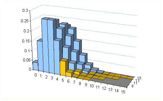
For a given N the
sum of histograms marked in yellow ![]() is the probability of
having more than
is the probability of
having more than ![]() erasures, i.e. the
probability of decoding failure at the receiver.
erasures, i.e. the
probability of decoding failure at the receiver.
These probabilities are plotted on the chart below.
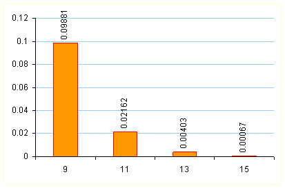
If our objective (in the same example with ![]() and
and ![]() ) is to have a DER below 1%, we can transmit the media in
blocks of 13 packets (containing 8 redundant packets).
) is to have a DER below 1%, we can transmit the media in
blocks of 13 packets (containing 8 redundant packets).
For a given M and DER we need a fast method for computing the minimal required N needed for successful media streaming at network’s random loss probability p.
III.
Fast
computation of Binomial Distribution
The below representation of binomial contains less multiplications and divisions and we have no components containing very large numbers and therefore have less precision errors:

![]()
![]()
Additional speedup is obtained by applying the above method for
computing the binomial only at ![]() and by obtaining the
remaining values of the binomial, iteratively, from the value computed at k:
and by obtaining the
remaining values of the binomial, iteratively, from the value computed at k:

Below is an implementation of the algorithm in AMPL:
|
reset; param ver symbolic =
"a46a"; param p; param q=1-p; param N; param k=round(N*p); param pq= if k in interval [1,N/2] then p*q^((N-k)/k) else if k in interval (N/2,N-1] then
p^(k/(N-k))*q ; param Bk=
if k==0 then q^N else
if k==N then p^N else
if k in interval [1,N/2] then
prod{i in 1..k} ((N-k+i)/i*pq) else
if k in interval (N/2,N-1] then prod{i in 1..N-k} ((k+i)/i*pq) ; param Binomial{n in 0..N} =
if n=k then Bk
else if n>k then Binomial[n-1]*(N-n+1)/n*p/q
else if n<k then Binomial[n+1]*(n+1)/(N-n)*q/p; data; param N=20; param p=0.3; model; param file symbolic = ver &
"-out.csv"; printf ",Binomial
Distribution\n" > (file); for{n in 0..N} {
printf "%d,%.20f\n",n,Binomial[n] > (file); } close (file); |
IV.
Computing
the minimally needed length of the transmitted codeword for maintaining the
decoding failure probability satisfactorily low
The decoding failure probability for a given N is always more than ![]()
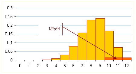
Binomial distribution for ![]() ,
, ![]() ,
, ![]()
Therefore the lower bound for N seeking a failure probability less than or equal to DER is:
![]()
From the other side if for a given ![]()
![]()
Then ![]()
Binomial distribution with ![]() ,
, ![]() ,
, ![]()
The upper bound ![]() for N is chosen as the smallest from
sequence
for N is chosen as the smallest from
sequence ![]() , for which
, for which ![]() :
:
![]()
such that:

For every ![]() in the interval from
the lower bound to the upper bound, we compute the exact value of the failure
probability, and chose the lowest N
at which the failure probability is below DER.
in the interval from
the lower bound to the upper bound, we compute the exact value of the failure
probability, and chose the lowest N
at which the failure probability is below DER.
Below is an implementation of the algorithm in AMPL:
|
reset; param
ver symbolic = "a73a"; param
M integer >=1; param
DER; set
P within interval [0,1] = setof{p in 0..0.9 by 0.001} round(p,10); param
param
maxN_probe{p in P, pr in 1..4} = param
Binomial_probe{p in P, pr in 1..4} = if M>=2 then prod{i in 1..M-1} ( (maxN_probe[p,pr]-M+1+i)/i * p^((maxN_probe[p,pr]-M+1)/(M-1))*(1-p) ) else p^maxN_probe[p,pr]; param
maxN{p in P} = maxN_probe[p, min{pr in 1..4: Binomial_probe[p,pr]<=DER/M}
pr]; set
NN{p in P} = { param
Binomial1{p in P, Ntr in NN[p]}= if M>=2 then prod{i in
1..M-1}((Ntr-M+1+i)/i*p^((Ntr-M+1)/(M-1))*(1-p)) else p^Ntr; param
pbyq{p in P} = p/(1-p); param
Binomial{p in P, Ntr in NN[p], n in Ntr-M+1..Ntr} = if n=Ntr-M+1 then Binomial1[p,Ntr] else Binomial[p,Ntr,n-1]*(Ntr-n+1)/n*pbyq[p]; param
Failure{p in P, Ntr in NN[p]} = sum{i in Ntr-M+1..Ntr}Binomial[p,Ntr,i]; param
goodN{p in P} = min{Ntr in NN[p]: Failure[p,Ntr]<=DER} Ntr; param
file symbolic = ver & "-out.csv"; let
DER := 1e-5; param
log symbolic = "benchmark.log"; param
benchmark_rec symbolic; param
benchmark_start; param
benchmark_stop; let
benchmark_start := _ampl_time; printf
"Version %s:\n",ver; printf
",FEC\n" > (file); for{m
in 1..15} { let M := m; print M, DER; for{p in P} { printf "%f,%f\n",p, goodN[p]/M > (file); } printf "\n" > (file); } close
(file); let
benchmark_stop := _ampl_time; let
benchmark_rec := sprintf("%s, %s, done in %f seconds", sub(ctime(),"^[^ ]*
*",""),ver,benchmark_stop-benchmark_start); print
benchmark_rec; print
benchmark_rec >> (log); close (log); |
Codeword overheads as functions from random loss probability are plotted for various numbers of media packets in the block:
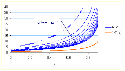
The smallest values of N
at which the decoding failure probability is still below ![]() for all M in {1..15}.
for all M in {1..15}.
The orange curve represents the overhead of an ideal communication
that reached its
V.
Interpolation
Instead of an integer codeword length function of p, we would like to have a curve
crossing smoothly also the non integer values between two ![]() and N.
and N.
Let us remind that N
is chosen such that the failure probability at N is below DER and at ![]() is above:
is above:
![]()
The failure probabilities for N and ![]() are known and already computed.
are known and already computed.
We know that the lower bound of ![]() is
is ![]() (when
(when ![]() , it is an exact value). Considering the shape of the lower
bound
, it is an exact value). Considering the shape of the lower
bound ![]() as sufficiently good
approximation, we thus will chose a similar function for finding the real value
x between two integers
as sufficiently good
approximation, we thus will chose a similar function for finding the real value
x between two integers![]() and N, at which
“length” the failure probability is supposedly equal exactly to DER.
and N, at which
“length” the failure probability is supposedly equal exactly to DER.
For two failure probabilities at N and ![]() we may say
we may say
![]()
![]()
where ![]() and
and ![]() are some accordingly
chosen values for the two probabilities at
are some accordingly
chosen values for the two probabilities at ![]() and N
and N
Precisely the values of ![]() and
and ![]() are the following:
are the following:
![]()
![]()
But as we will see below we will not need to refer to the
values of ![]() and
and ![]() :
:
The real value![]() is computed to respect the same interpolation:
is computed to respect the same interpolation:
![]()
![]()
![]()
![]()
![]()
![]()
![]()
![]()
![]()
Here is the corresponding AMPL plug-in to be added to the previous script:
|
param
codeword{p in P} = if goodN[p]-1 in NN[p] and
Failure[p,goodN[p]-1]>DER then goodN[p]-1 + (log(Failure[p,goodN[p]-1]) -
log(DER)) / (log(Failure[p,goodN[p]-1]) - log(Failure[p,goodN[p]])) else goodN[p]; |
The full text of the AMPL script is here.
Just for a comparison, the below chart compares the above obtained logarithmical interpolation with this the following linear formula for x, whose curve has much worst shape.
![]()
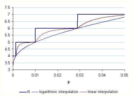
Codeword size to be transmitted for satisfying![]() with
with ![]()
Below are smoothened curves of required codeword sizes for
various M. The orange curve is the theoretical
lower bound resulted from the
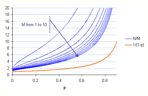
VI.
A
coarse approximation
The codeword overhead ![]() can be quite well
approximated with
can be quite well
approximated with

where c is some constant (see an excel file)
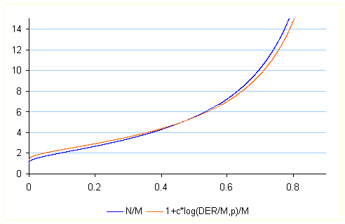
Codeword overhead ![]() for
for ![]() with
with ![]() and
and ![]()
* * *
© 2005, Switzernet (www.switzernet.com)